isolateContribution

Environmental time-series signal processing: Contribution isolation based on background subtraction, deseasonalisation and/or deweathering.

Usage

isolateContribution(
  data,
  pollutant,
  background = NULL,
  deseason = TRUE,
  deweather = TRUE,
  method = 2,
  add.term = NULL,
  formula = NULL,
  use.bam = FALSE,
  output = "mean",
  ...
)

Arguments

data: Data source, typically data.frame (or similar), containing all time-series to be used when applying signal processing.
pollutant: The column name of the data time-series to be signal processed.
background: (optional) if supplied, the background time-series to use as a background correction. See below.
deseason: logical or character vector, if TRUE (default), the pollutant is deseasonalised using day.hour and year.day frequency terms, all calculate from the data time stamp, assumed to be date in data. Other options: FALSE to turn off deseasonalisation; or a character vector of frequency terms if user-defining. See below.
deweather: logical or character vector, if TRUE (default), the data is deweathered using wind speed and direction, assumed to be ws and wd in data). Other options: FALSE to turn off deweathering; or a character vector of data column names if user-defining. See below.
method: numeric, contribution isolation method (default 2). See Note.
add.term: extra terms to add to the contribution isolation model; ignore for now (in development).
formula: (optional) Signal isolate model formula; this allows user to set the signal isolation model formula directly, but means function arguments background, deseason and deweather will be ignored.
use.bam: (logical) If TRUE, the bam is used instead of standard gam to build the model.
output: output options; currently, 'mean', 'model', and 'all'; but please note these are in development and may be subject to change.
...: other arguments; ignore for now (in development)

Value

isolateContribution returns a vector of predictions of the pollutant time-series after the requested signal isolation.

Details

isolateContribution estimates and subtracts pollutant variance associated with factors that may hinder break-point/segment analysis:

Background Correction If applied, this fits the supplied background time-series as a spline term: s(background).
Seasonality If applied, this fits regular frequency terms, e.g. day.hour, year.day, as spline terms, default TRUE is equivalent to s(day.hour) and s(year.day). All terms are calculated from date column in data.
Weather If applied, this fits time-series of identified meteorological measurements, e.g. wind speed and direction (ws and wd in data). If both ws and wd are present these are fitted as a tensor term te(ws, wd). Other deweathering terms, if included, are fitted as spline term s(term). The default TRUE is equivalent to te(ws, wd).

Using the supplied arguments, it builds a signal (mgcv) GAM model, calculates, and returns the mean-centred residuals as an estimate of the isolated local contribution.

Note

method was included as part of method development and testing work, and retained for now. Please ignore for now.

References

Regarding mgcv GAM fitting methods, see Wood (2017) for general introduction and package documentation regarding coding (mgcv):

Wood, S.N. (2017) Generalized Additive Models: an introduction with R (2nd edition), Chapman and Hall/CRC.

Regarding isolateContribution, see:

Ropkins, K., Walker, A., Philips, I., Rushton, C., Clark, T. and Tate, J., Change Detection of Air Quality Time-Series Using the R Package AEQval. Available at SSRN 4267722. https://ssrn.com/abstract=4267722 or http://dx.doi.org/10.2139/ssrn.4267722 Also at: https://karlropkins.github.io/AQEval/articles/AQEval_Intro_Preprint.pdf

Author

Karl Ropkins

Examples

#fitting a simple deseasonalisation, deweathering
#and background correction (dswb) model to no2:

aq.data$dswb.no2 <- isolateContribution(aq.data,
                        "no2", background="bg.no2")
#> no2 ~ s(bg.no2) + te(wd, ws) + s(year.day) + s(day.hour)

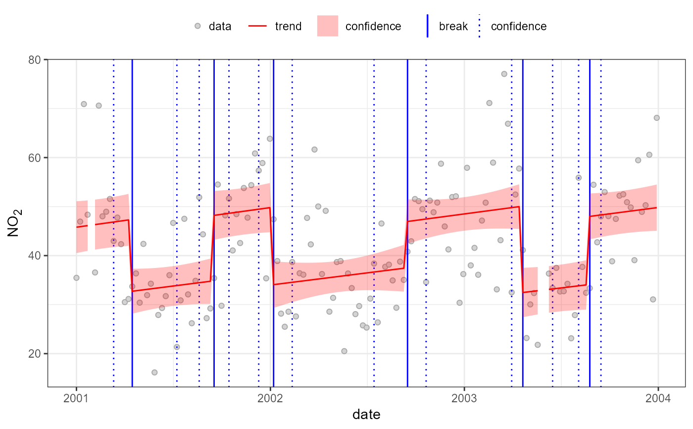
#compare at 14 day resolution:
temp <- openair::timeAverage(aq.data, "14 day")

#without dswb
quantBreakPoints(temp, "no2", test=FALSE, h=0.1)
#> Using all 6 suggested breaks
#> 
#> 2001-03-26 (2001-02-26 to 2001-07-02)
#> 49.03->33.34;-15.69 (-32%)
#> 
#> 2001-09-24 (2001-09-10 to 2001-10-22)
#> 34.57->48.63;14.05 (41%)
#> 
#> 2001-12-31 (2001-11-19 to 2002-01-14)
#> 49.35->35.78;-13.57 (-27%)
#> 
#> 2002-09-09 (2002-07-29 to 2002-11-04)
#> 37.53->46.77;9.234 (25%)
#> 
#> 2003-04-07 (2003-03-10 to 2003-05-05)
#> 48.36->34.63;-13.73 (-28%)
#> 
#> 2003-08-11 (2003-07-14 to 2003-08-25)
#> 35.41->47.95;12.54 (35%)


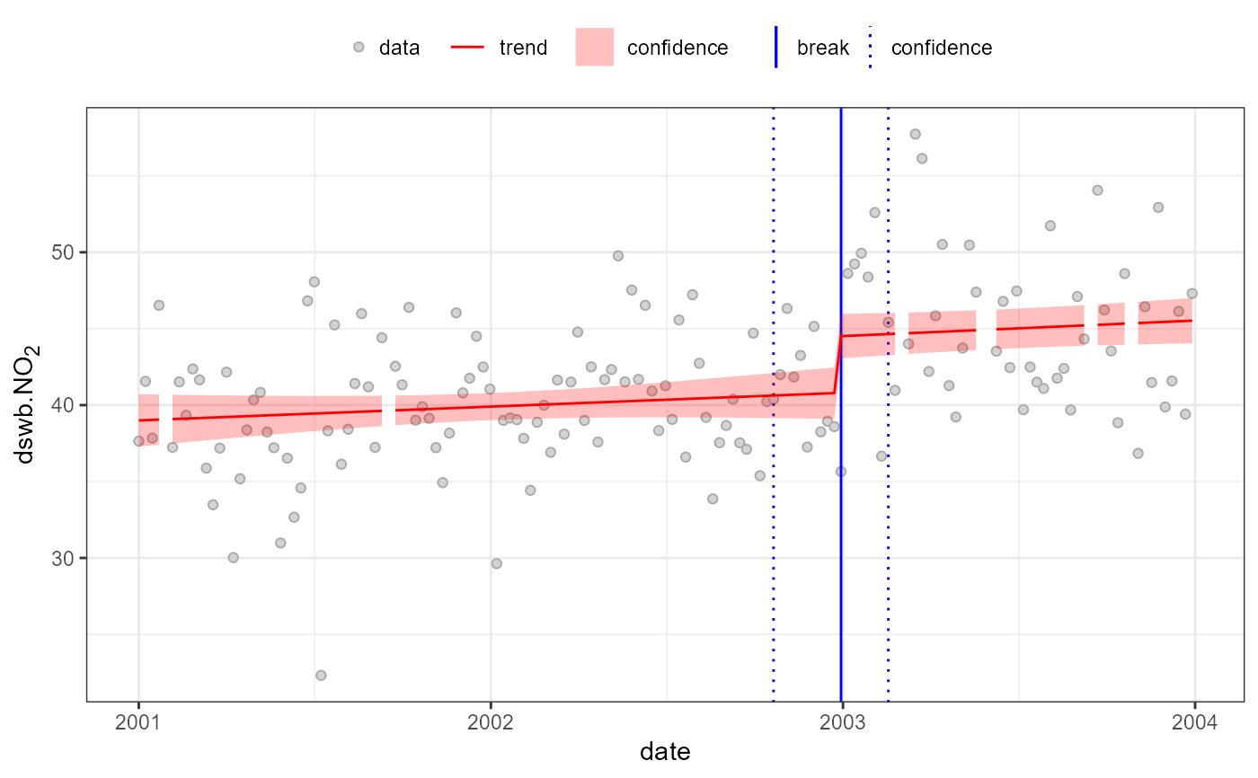
#with dswb
quantBreakPoints(temp, "dswb.no2", test=FALSE, h=0.1)
#> Using all 1 suggested breaks
#> 
#> 2002-12-30 (2002-10-07 to 2003-02-24)
#> 40.8->44.67;3.865 (9.5%)