quantify break-point/segments

Quantify either break-points or break-segment methods for pollutant time-series

Usage

quantBreakPoints(
  data,
  pollutant,
  breaks,
  ylab = NULL,
  xlab = NULL,
  pt.col = c("lightgrey", "darkgrey"),
  line.col = "red",
  break.col = "blue",
  event = NULL,
  show = c("plot", "report"),
  ...
)

quantBreakSegments(
  data,
  pollutant,
  breaks,
  ylab = NULL,
  xlab = NULL,
  pt.col = c("lightgrey", "darkgrey"),
  line.col = "red",
  break.col = "blue",
  event = NULL,
  seg.method = 2,
  seg.seed = 12345,
  show = c("plot", "report"),
  ...
)

Arguments

data: Data source, typically a data.frame or similar, containing data-series to model and a paired time-stamp data-series, named date.
pollutant: The name of the data-series to break-point or break-segment model.
breaks: (Optional) The break-points and confidence intervals to use when building either break-point or break-segment models. If not supplied these are build using findBreakPoints and supplied arguments.
ylab: Y-label term, by default pollutant.
xlab: X-label term, by default date.
pt.col: Point fill and line colours for plot, defaults lightgrey and darkgrey.
line.col: Line colour for plot, default red.
break.col: Break-point/segment colour for plot, default blue.
event: An optional list of plot terms for an event marker, applied to a vertical line and text label. List items include: x the event date (YYYY-MM-DD format) require for both line and label; y by default 0.9 x y-plot range; label the label text, required for label; line.size the line width, by default 0.5; font.size the text size, by default 5; and, hjust the label left/right justification, 0 left, 0.5 centre, 1 right (default). See also examples below.
show: What to show before returning the break-point quantification mode, by default plot and report.
...: other parameters
seg.method: (quantBreakSegments only) the break-segment fitting method to use.
seg.seed: (quantBreakSegments only) the seed setting to use when fitting break-segments, default 12345.

Value

Both functions use the show argument to control which elements of the functions outputs are shown but also invisible return a list

of all outputs which can caught using, e.g.:

brk.mod <- quantBreakPoints(data, pollutant)

Details

quantBreakPoints and quantBreakSegments both use strucchange methods to identify potential break-points in time-series, and then quantify these as conventional break-points or break-segments, respectively:

Finding Break-points Using the strucchange methods of Zeileis and colleagues and independent change detection model, the functions apply a rolling-window approach, assuming the first window (or data subset) is without change, building a statistical model of that, advancing the window, building a second model and comparing these, and so on, to identify the most likely points of change in a larger data-series. See also findBreakPoints
Quantifying Break-points Using the supplied break-points to build a break-point model.
Quantifying Break-segments Using the confidence regions for the supplied break-points as the starting points to build a break-segment model.

Note

AQEval function quantBreakSegments is currently running segmented v.1.3-4 while we evaluate latest version, v.1.4-0.

References

Regarding strucchange methods see in-package documentation, e.g. breakpoints, and:

Achim Zeileis, Friedrich Leisch, Kurt Hornik and Christian Kleiber (2002). strucchange: An R Package for Testing for Structural Change in Linear Regression Models. Journal of Statistical Software, 7(2), 1-38. URL https://www.jstatsoft.org/v07/i02/.

Achim Zeileis, Christian Kleiber, Walter Kraemer and Kurt Hornik (2003). Testing and Dating of Structural Changes in Practice. Computational Statistics & Data Analysis, 44, 109-123. DOI doi:10.1016/S0167-9473(03)00030-6 .

Regarding segmented methods see in-package documentation, e.g. segmented, and:

Vito M. R. Muggeo (2003). Estimating regression models with unknown break-points. Statistics in Medicine, 22, 3055-3071. DOI 10.1002/sim.1545.

Vito M. R. Muggeo (2008). segmented: an R Package to Fit Regression Models with Broken-Line Relationships. R News, 8/1, 20-25. URL https://cran.r-project.org/doc/Rnews/.

Vito M. R. Muggeo (2016). Testing with a nuisance parameter present only under the alternative: a score-based approach with application to segmented modelling. J of Statistical Computation and Simulation, 86, 3059-3067. DOI 10.1080/00949655.2016.1149855.

Vito M. R. Muggeo (2017). Interval estimation for the breakpoint in segmented regression: a smoothed score-based approach. Australian & New Zealand Journal of Statistics, 59, 311-322. DOI 10.1111/anzs.12200.

Regarding break-points/segment methods, see:

Ropkins et al (In Prep).

Author

Karl Ropkins

Examples

#using openair timeAverage to covert 1-hour data to 1-day averages

temp <- openair::timeAverage(aq.data, "1 day")

#break-points

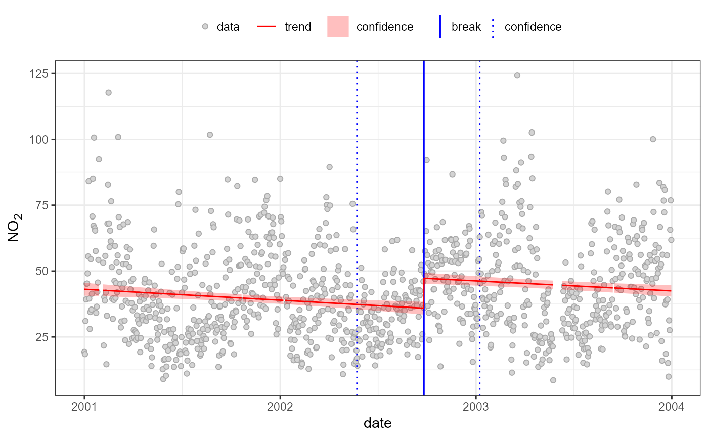
quantBreakPoints(temp, "no2", h=0.3)
#> Using 1 of 1 suggested breaks: 1
#> 
#> 2002-09-26 (2002-05-24 to 2003-01-08)
#> 35.93->47.28;11.35 (32%)


#break-segments

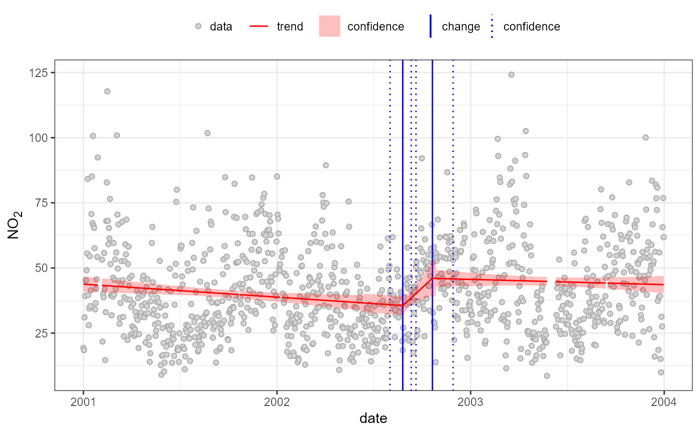
quantBreakSegments(temp, "no2", h=0.3)
#> Using 1 of 1 suggested breaks: 1
#> building 3 segments
#> 
#> 2001-01-01 to 2002-08-26 (602)
#> 43.78->35.57;-8.208 (-18.75%)
#> 
#> 2002-08-26 to 2002-10-21 (56)
#> 35.57->46.02;10.44 (29.35%)
#> 
#> 2002-10-21 to 2003-12-31 (436)
#> 46.02->43.61;-2.406 (-5.23%)


#addition examples (not run)
if (FALSE) {
#in-call plot modification
#removing x axis label
#recolouring break line and
#adding an event marker
quantBreakPoints(temp, "no2", h=0.3,
       xlab="", break.col = "red",
       event=list(label="Event expected here",
                 x="2002-08-01", col="grey"))
}